The following figure illustrates index sequential sets and subsets.

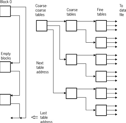
An index sequential set or subset is a collection of tables arranged hierarchically. At the lowest level of the hierarchy are fine tables. One entry exists in the fine tables for each data set record contained in the set or subset. Within any table, entries are kept in increasing binary collating sequence. This enables a binary search to be performed within any table.

Fine tables are ordered by another level of tables called coarse tables. One entry exists in the coarse tables for each fine table. If there are more fine tables than can be indexed by a single coarse table, then several coarse tables are created and these tables are ordered by a coarse-coarse table. This hierarchy continues until there is only one table at the top level in the disjoint case, or one table for each master in the embedded case. The system permits as many as 22 levels of tables; but, in practice, there are seldom more than three or four levels.

The maximum number of levels of tables available can be determined using the following calculation:

45 DIV (n+1)

The variable n represents the number of bits that it would take to represent the table size in binary form.

The following table shows a range of that calculation.

Initially, there is only one fine table containing only an Omega entry. The Omega entry is a system-created dummy key entry consisting of the highest key value (all ones). The Omega entry can never be deleted.

Since entries are always maintained in sequence, a new entry must be placed in a particular position. To find that position, a FIND AT operation is implicitly performed. If there is room in the proper table, the entry is inserted there and the entries ahead of it are moved up. If there is no room, then a table split is performed by allocating a new table, moving some of the entries from the old table to the new table, and adding an entry for the new table in the next higher level of tables.

The number of entries moved from the old to the new table depends upon both the LOADFACTOR value and where the new entry goes. The following figure gives a graphic interpretation of the movement of entries.

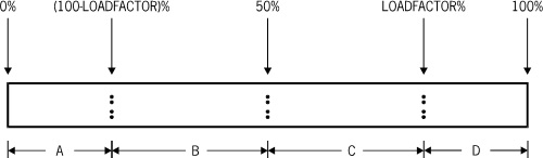
Effect of LOADFACTOR Value on Entry Movement details the movement of entries.

It should be noted that the split point is always computed in entries, thus an individual entry is never split between tables. Since tables are split based upon the location of new entries, loading in serial order results in an average loading of LOADFACTOR percent.

If the single table at the highest level must be split, then a new level is added to the hierarchy. That is, the hierarchy goes from one level of tables to two, from two levels to three, and so on. The new table added at the highest level is used to index the tables resulting from the split. The number of levels grows equally for the structure since the new table is added at the top. For example, if the fine tables were previously one level from the top, they will all henceforth be two levels from the top.

Once the number of levels increases, it never decreases. This is the case since Omega entries exist at each level, even if all other key entries are deleted. The Reorganization process can, of course, be used to re-create the structure entirely and thus eliminate levels.

For disjoint sets and subsets, the highest level table is always the second block of the file. For embedded sets and subsets, the highest level table for a given master never moves; it always has the same block address no matter how many times a level grows. As a result, the address in the master need never be adjusted.

Notice that tables are only split when they are full and a new entry must be inserted. For the embedded case, a split under one master does not cause a split under others.

The more levels a table has, the less efficient it is in finding a table entry. A garbage collection is recommended if table levels grow to four or more levels.