A physically sectioned index sequential set divides a set structure in multiple physical files. Each physical file represents a single section, and every section has its own root table. Block 1 in section 0 (zero) is the section table and looks similar to a typical root table except that it is the entry point to the multiple physical roots. For a physically sectioned set or subset, the section table can actually span multiple blocks in different physical files, even though it is still considered the main root.
If the section table exceeds the standard TABLESIZE value, blocks are linked together to form a single-root section table just as they are in logically sectioned sets. This is all controlled by a single bit in block 0 (zero). If the file is sectioned, bit [16:1] of the table control word in block 0 is on, which indicates that block 1 in section 0 is a section table as opposed to a root table for a nonsectioned set or subset.
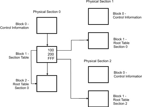
The following figure shows the file layout of the sectioned set with multiple files. Each section is an independent file. The section table is in block 1 of section 0. The root table resides in each section.
The following figure illustrates the table control word of block 1 for a sectioned file.
Example 38. Table Control Word of Block 1
A    47: 28
     BAF link to additional section table blocks. If zero, this is the last
     block of the section table.
B    16: 1
     Value=1. This it the section table of a sectioned set.
C    15:15
     Number of entries in this block of the section table.
D    0:1
     Value=1. This is a fine table of a section table.
The entries in a section table look like entries in any other coarse table. The key value represents the upper limit of the keys below, and the AA word points to the root for a given section.
DASDL specifications for sectioning sets determine what the sections look like when the file is initialized by DMUTILITY. All sectioning information for an index sequential set or subset is contained within the file and determines how the set or subset file is logically sectioned.
Table Format
The following figure illustrates the table format for index sequential sets and subsets.
Example 39. Index Sequential Set and Subset Table Format
            WORD
              0      Table control word (TCW)
              1      Table serial number (TSN)
              2      ---
                      .
                      .   Unused key entries.
                      .
                     ---
                     ---
                      .
                      .   In-use key entries in
                      .   ascending sequence.
                      .   (First entry is numbered one.)
                      .
                     ---
                     ---
                      .
                      .   Unused key entries.
                      .
                     ---
Valid entries are always contiguous within tables. Within the range of valid entries, the entries are always in order by key, thus allowing a binary search to be used for insertion and retrieval. Entries are allowed to float within tables under the control of TCWs. Once the entries reach the beginning of the table, they are moved down to the end of the table. Each TCW gives the location of the first entry, indicates the number of entries, and indicates whether the table is coarse or fine. Refer to “Common Features” earlier in this appendix for layout details. For coarse tables, the AA words point to other tables in the set; for fine tables, they point to records in the data set.
If the database is audited, the TSN is used to coordinate the current state of the table with the audit trail. In unaudited databases, the TSN is present but not used.
Empty blocks arise from deleting all entries in a table. These blocks are kept in a one-way linked list whose head is in block 0 (zero).
Index Sequential Set and Subset Restrictions
For the following reasons there are no restrictions on index sequential sets and subsets:
-
Efficient disk space utilization depends upon keeping tables reasonably full. When the set or subset is initially loaded in either ascending or descending sequence, tables are LOADFACTOR percent full. Random additions can cause the average table loading to change. Reorganization can be used to reorder and compact the index sequential structures.
-
Tables for embedded structures are not shared between masters. Since the minimum table size is one segment, at least one segment is allocated for each master with details.
-
FIND NEXT and FIND PRIOR operations access entries sequentially within each fine table, and then examine the coarse tables to locate the next fine table. Thus, the operations are extremely fast. The path for an index sequential structure includes not only the fine table but also the current coarse tables for each level of the hierarchy. Entries are returned in order by key.
-
A FIND AT operation uses a binary search at each table level and is efficient. Although one table is accessed at each level, the buffer management scheme chooses the least frequently used tables to overlay; the result is that the coarse tables tend to remain in memory if sufficient buffers are allocated.
-
When a record in a data set is created or deleted, spanning index sets are updated in the order in which they are declared in the DASDL description. (Note that lock and store operations that change the key also cause index sets to be updated.) Fine tables that are affected are locked and remain locked until all the updates are complete. If the contention on the fine tables of the first spanning set caused by serial updating minimizes the throughput, and if the spanning set is declared last in the DASDL description and other indexes are accessed randomly, performance can be improved.
-
Because the order in which fine tables are locked is based on the order of declarations in the DASDL description, it is beneficial if the most randomly distributed set is declared first and the least randomly distributed set is declared last.
-
The number of levels can be controlled using the TABLESIZE and LOADFACTOR values, and can be computed as follows:
((TABLESIZE * LOADING) ** N) GEQ POPULATION
The elements of the equation are explained in the following text:
|
Element |
Description |
|---|---|
|
LOADING |
Average number of entries for each table divided by TABLESIZE. Initially this is LOADFACTOR if the structure is loaded in sequence. |
|
N |
Number of table levels. |
|
POPULATION |
Total number of entries. |
The equation is equivalent to the Nth root of the POPULATION value divided by the LOADING value, which can be expressed as
TABLESIZE GEQ (POPULATION ** (1/N)) / LOADING
For example, assume a POPULATION of 10,000 and a LOADING of 66.7 percent; then the TABLESIZE values when there are two and three levels of tables are greater than or equal to 150 and 33 respectively. The calculation for the TABLESIZE value when there are two levels of tables is as follows:
     TABLESIZE  GEQ  (10,000 ** (1/2)) /.667
           GEQ  100/.667
           GEQ  150
The TABLESIZE value calculation when there are three levels of tables is as follows:
   TABLESIZE GEQ  (10,000 ** (1/3)) /.667
         GEQ  22/.667
         GEQ  33
Since one I/O operation can be required for each table level, random access is generally faster when tables are reasonably large, resulting in fewer levels of tables. However, a large TABLESIZE value requires more I/O transfer time, more core space, and more processor overhead to move entries during an update. Therefore, if the TABLESIZE value is so large that it costs more to maintain one large table than two smaller ones, the structure should be designed with a smaller TABLESIZE value and more levels.
